As an SEO, I heavily rely on Google Sheets to automate my work and enhance efficiency. In this article, I’ll share five functions that I use in Google Sheets for SEO tasks. Even if you’re not an SEO, you may still find this article beneficial. I encourage you to keep reading. We’ll start with a function that allows you to extract and manipulate parts of URLs, and conclude with a function that enables you to gather information such as titles, meta descriptions, or even headings from large numbers of URLs. While the focus is on five main functions, stay tuned for a bonus function at the end of this article. Let’s begin with the Split function.
1 – Split: Extract and Manipulate Parts of URLs
Imagine you have a list of thousands of URLs, and you want to better understand the site’s architecture, or in some cases, you want to just get a specific part of the URL like categories, or you might want to remove something like a UTM from a list of URLs. Split is the function that can help you in this case.
The function has this structure:
=SPLIT(text, delimiter, [split_by_each], [remove_empty_text])To use it, you need to at least define two things, first is text (The text to divide.) which in our case is the URL and the second is delimiter(The character or characters to use to split text) which in this example is most of the times the “/” character. But you might need other delimiters based on your need. Keep in mind that you need to put the delimiter character between two “ characters.
The screenshot below shows how I could split the UTM section from the list of URLs with this simple formula “=split(A2,”?”)”

2- CONCATENATE and Ampersand: Build and Combine URLs
Sometimes, you may need to create a list of URLs, whether to build a sitemap, suggest a structure for a new website, or create a list of UTM URLs. Additionally, if a website is migrating to a new domain, you might need to generate a list of redirects to pair each old URL with its new destination, among many other possible uses. In such situations, the CONCATENATE function is highly useful.
The function has this structure:
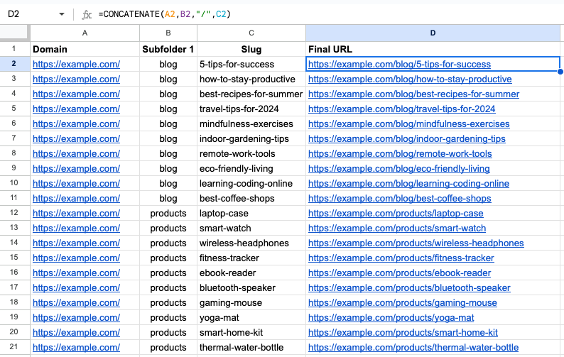
=CONCATENATE(text1, text2, text3 ,....)To use it, you need at least two cells containing text. Simply include the text or the cells containing the text in your formula. In the example below, you can see how I combined a domain, subfolder, and slug using “=CONCATENATE(A2, B2, “/”, C2)” to create a list of URLs. It’s important to note that you must manually include any separators; in this case, I added the “/” character myself.
Another method to achieve the same result is using the “&” operator. For example, the formula “=A2 & B2 & “/” & C2” will combine the same elements into a full URL.
3- VLOOKUP: Quickly Match and Retrieve SEO Data Across Sheets
VLOOKUP is incredibly useful when you need to find and correlate data across different sheets. For example, you might have one sheet with URLs, clicks, and impressions and another with URLs and Page Speed Insight scores. With VLOOKUP, you can match data between these sheets based on URLs, allowing you to create a combined sheet that includes URLs with their clicks, impressions, and PSI scores.
The function has this structure:
=VLOOKUP(search_key, range, index, [is_sorted])To use this function, you need two sets of data with a common element, known as the “search_key.” Google Sheets uses this key to match data and find what you need between two datasets.
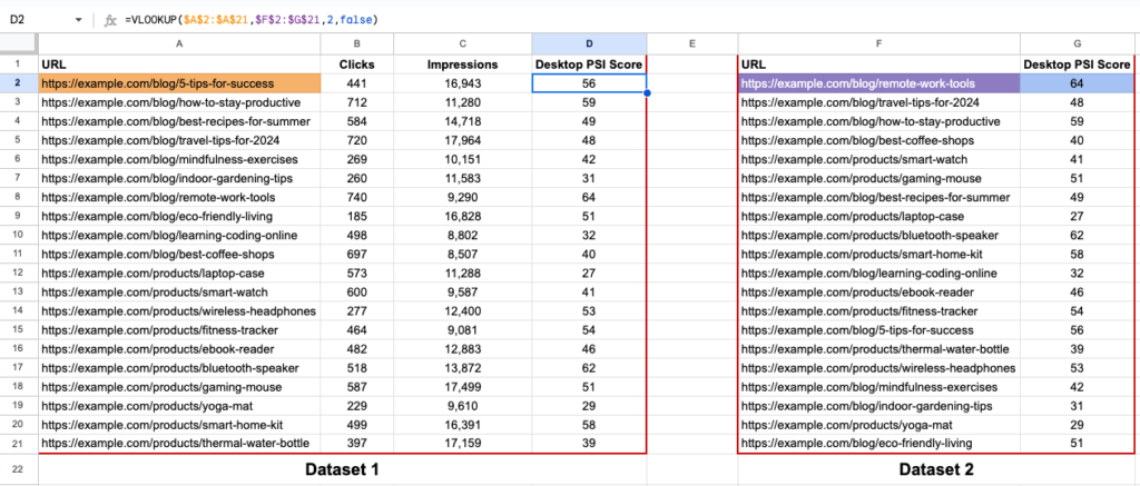
In the example below, I have two sets of data, with the URLs in common as the search key. I’m getting the search key from dataset 1 in the range A2:A21. The next element to specify is “range,” which is the area where you want to look for the search key; in this example, it is F2:G21. Next, define the “index,” which is the column number in the range from which you want to retrieve the value. In this example, it’s from column G of the range, which is the second column, meaning the index will be “2”. Lastly, we have the optional parameter [is_sorted], which you can set to FALSE to ensure an exact match.
The screenshot below demonstrates how we could retrieve the Desktop PSI score from the second dataset and match it with the correct URL in the first dataset using VLOOKUP. The usage is not limited to this example, and there are infinite possibilities for applying this function.
4 – ARRAYFORMULA: Automate Data Operations Across Multiple Rows
When working with large datasets, you might initially think to paste a formula into thousands of cells, typically by dragging the formula down to the desired cell. However, a more efficient method is to use ARRAYFORMULA to perform bulk operations on a range of data without the need to drag formulas across multiple rows. A significant advantage of using this function is that if you need to make any changes to your formula, you can simply modify it in one cell, and the changes will apply to the entire range, eliminating the need to drag and update each cell individually.
The function has this structure:
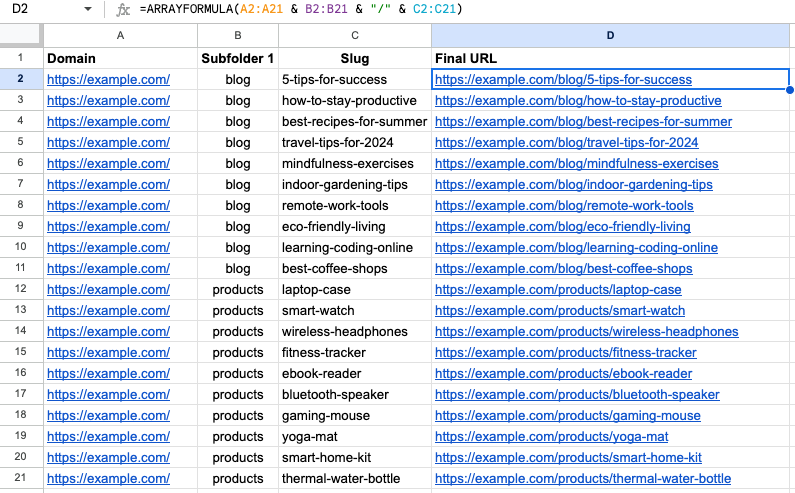
=ARRAYFORMULA(array_formula)In the example below, we use the & operator with ARRAYFORMULA to avoid pasting the formula in all cells. Thus, the formula is only entered once in cell D2.
In the example below, we use the & operator with ARRAYFORMULA to avoid pasting the formula in all cells. Thus, the formula is only entered once in cell D2.
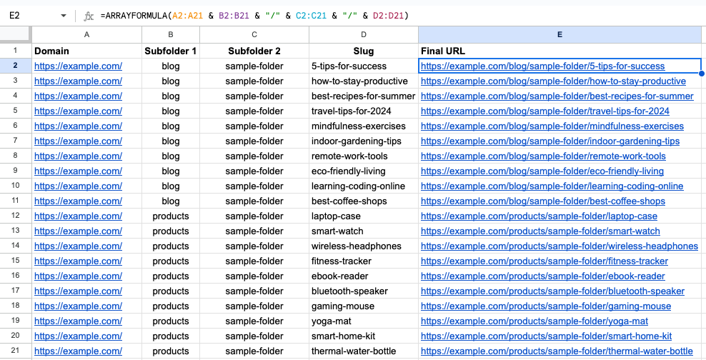
In the screenshot below, you can see that when I decided to add a second subfolder to the URL, I just added it to the E2 cell, and without needing to make any further changes, all cells in column E were automatically updated.
5 – IMPORTXML: Fetch and Integrate Web Data Directly Into Google Sheets
When you need to extract specific data from web pages, IMPORTXML can be your best friend. Imagine you have a list of 100 URLs, and you want to retrieve all H1 tags, Titles, meta descriptions, or any other common element across these URLs. This function allows you to efficiently gather the data you need.
The function has this structure:
=IMPORTXML(url, xpath_query)To use IMPORTXML, you need two components: the URL of the page and the xpath_query for the element you are looking for. It works well on many websites, but if access is restricted on a specific domain, you might not be able to use this function for some sites.
In the example below, I extracted titles, meta descriptions, and the first H2 elements from 10 blogs on SEMrush.
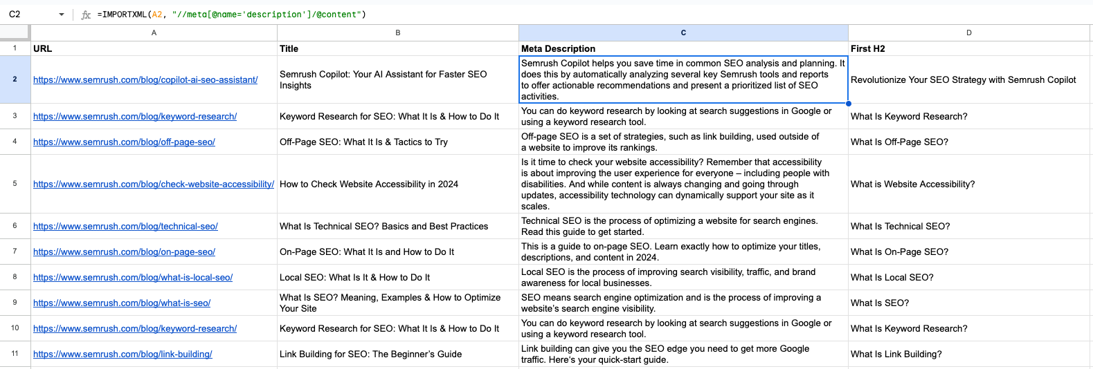
To get the title, I used:
=INDEX(IMPORTXML(A2, "//title"), 1)For meta descriptions:
=IMPORTXML(A2, "//meta[@name='description']/@content")And for the first H2:
=INDEX(IMPORTXML(A2, "//h2"), 1)Here we have a bonus function to explain, INDEX. The INDEX function allows you to select a specific element from a set of results or from a specific array position. It’s particularly useful when IMPORTXML returns multiple results, and you need to pinpoint a single item.
Continuing the Conversation: Share Your Insights
There are many other ways to automate tasks with Google Sheets, and I plan to write more on this topic in the future. For now, you might also want to check out a tool I’ve developed using Google Sheets and AppScript to cluster large groups of keywords, which you can purchase on Gumroad. I always enjoy automating tasks using various tools and sharing my knowledge and experiences with you. If you’d like to learn more about the other ways I automate my tasks as an SEO, let me know—I would be happy to share more. Also, if you use any other functions that enhance your performance, feel free to share them in the comments section.
